Write Up 3: Roots of Quadratics

Graphs in the XB plane:

In this write up, we will be discussing the appearance and behavior of quadratic roots in the XB-plane. For this investigation, we will fix our constant "a=1" and for the first part of our investigation we will fix "c=1."

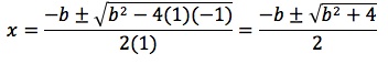
Let observe the equation in the XB- plane and take a look at its graph:

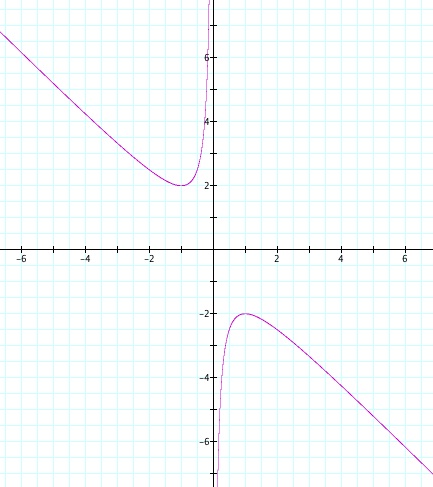
Let's observe that in order to have "real" solution to our equation, the value of "b" must be greater than 2 or less than 2. This is why we see two separate curves because if the value of "b" is between 2 and -2, then we will get imaginary roots leading to imaginary solutions. We can see this when using the quadratic formula. Let b=1, therefore we have:

As we can see, the solutions to our XB equation contain an "i" causing the the gap in our graph where the two curves do not touch.

Behavior of Quadratic Roots

Let's discuss the difference in solutions to our equation by observing the below media which shows how the solutions change given different values for "b."

The position of the red horizontal line determines how many roots we have to our quadratic equation . The first case is when the red horizontal line value becomes greater than 2 or less than -2, we have two real roots. More specifically, if b > 2 then we have two negative real roots and when b < 2 we have two positive real roots. This can be see when the red line intersects a the graph at two point represent the two real roots to our equation. The second case is when the red horizontal line equals 2 or -2. In this case, our horizontal line intersect the graph at only one point meaning that our quadratic equation gives us a one real root and a repeating solution. There are two points where this happens in our graph, which can be represented on the graph where the red line intersect the vertex of both curves. The third and final case shows the red horizontal line in between the two curves of our graph. When the red line is in this graph, there are zero intersection points which tells us that there are zero real roots and no real solutions. We discussed earlier that this gap in our graph represents imaginary solutions to our quadratic equation.

Vertical Shift Change in the Variable "c"

Now let observe what happens to our quadratic equation when we change the values for "c." The below graph represents graph of our quadratic equations with c=1, c=3, c=5, c=7:

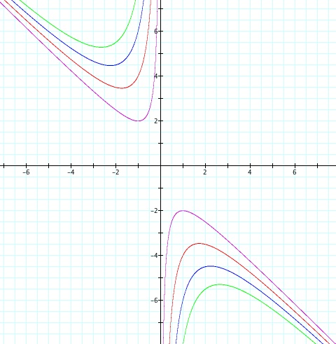
From the graph, we can see that the value of "c" controls our vertical shift of the two curves. We can also see that the the gap of imaginary solutions increases as the value of "c" increases and vise versa. We can see this increase of gap by comparing the gap between the purple curves and the gap between the green curves. The gap for imaginary solutions is much bigger when looking at the green curves compared to the gap between the purple curves. Also as "c" changes, the cases for quadratic equation's roots stays the same. Therefore regardless the value of "c" where "c0", we either have two real rots, one real root, or zero real roots. Again, it we were to drop a horizontal line into our above graph, the position of this graph would tell us the number of real roots we have depending on how many intersection points take place.

What If We Let C= -1?

Now lets consider the case when c= -1 rather than c=1. Hence, our new quadratic equation looks like . Let's see what the graph of this equation looks like as well:

Observe that the movable horizontal red line always touches the purple graphs at 2 point giving us two real roots. Now I want to talk about why we will "always" have two real roots when the value of "c=-1."Let's take a look at the quadratic formula when c=-1:

Let's focus on the stuff inside the radical which is . Since a square can never be negative and we have a positive four underneath the radical, then will will always have a positive number come out of the radical. To put it in better terms, cannot be negative meaning that we will always have two real roots regardless of the value of "b."

Conclusions

Lets looks at a graph with multiple values for ranging from -7< c < 7:

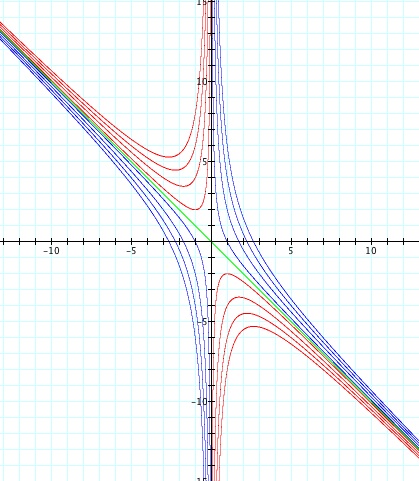
Let's observe that when the value of "c" does not equal zero, the corresponding graphs follow an asymptotic behavior. None of the graphs ever touch the line x=0 or the line x=-b. These two lines in the XB-plane acts as our asymptotes for this systems of graphs. Lets look at how these asymptotes are formed algebraically. If we set c=0 in our quadratic equation then we get the equation . Now we can solve for the variable x by using reverse distribution: x (x+b)=0. Therefore either x=0 or x=-b. These lines are represented in the above graph by the b-axis (or commonly known as the y-axis) and the lime green line.